Convert point environment data to a raster of majority-environment classes

Given point occurrences of environmental categories, classRast generates a raster grid with cell values specifying the majority environment therein.

Usage

classRast(grid, dat = NULL, xy, env, cutoff)

Arguments

grid: A SpatRaster to use as a template for the resolution, extent, and coordinate reference system of the returned object. Values can be empty.
dat: Either a data.frame or matrix for which xy and env are column names, or an empty argument.
xy: A vector specifying the name or numeric position of columns in dat containing coordinates, if dat is supplied, or a 2-column data.frame or matrix of coordinate values.
env: The name or numeric position of the column in dat containing a categorical environmental variable, if dat is supplied, or a vector of environmental values.
cutoff: The (decimal) proportion of incidences of an environmental category above which a cell will be assigned as that category. cutoff must be greater than 0.5.

Value

A raster of class SpatRaster defined by the terra package

Details

The cutoff threshold is an inclusive bound: environmental incidence proportions greater than or equal to the cutoff will assign cell values to the majority environmental class. For instance, if category A represents 65% of occurrences in a cell and cutoff = 0.65, the returned value for the cell will be A. If no single category in a cell meets or exceeds the representation necessary to reach the given cutoff, the value returned for the cell is indet., indeterminate. Cells lacking environmental occurrences altogether return NA values.

The env object can contain more than two classes, but in many cases it will be less likely for any individual class to attain an absolute majority the more finely divided classes are. For example, if there are three classes, A, B, and C, with relative proportions of 20%, 31%, and 49%, the cell value will be returned as indet. because no single class can attain a cutoff above 50%, despite class C having the largest relative representation.

Missing environment values in the point data should be coded as NA, not e.g. 'unknown'. classRast() ignores NA occurrences when tallying environmental occurrences against the cutoff. However, NA occurrences still count when determining NA status of cells in the raster: a cell containing occurrences of only NA value is classified as indet., not NA. That is, any grid cell encompassing original point data is non-NA.

Antell and others (2020) set a cutoff of 0.8, based on the same threshold Nürnberg and Aberhan (2013) used to classify environmental preferences for taxa.

The coordinates associated with points should be given with respect to the same coordinate reference system (CRS) of the target raster grid, e.g. both given in latitude-longitude, Equal Earth projected coordinates, or other CRS. The CRS of a SpatRaster object can be retrieved with terra::crs() (with the optional but helpful argument describe = TRUE).

References

Antell GT, Kiessling W, Aberhan M, Saupe EE (2020). “Marine biodiversity and geographic distributions are independent on large scales.” Current Biology, 30(1), 115-121. doi:10.1016/j.cub.2019.10.065 .

Nürnberg S, Aberhan M (2013). “Habitat breadth and geographic range predict diversity dynamics in marine Mesozoic bivalves.” Paleobiology, 39(3), 360-372. doi:10.1666/12047 .

Examples

library(terra)
# work in Equal Earth projected coordinates
prj <- 'EPSG:8857'
# generate point occurrences in a small area of Northern Africa
n <- 100
set.seed(5)
x <- runif(n,  0, 30)
y <- runif(n, 10, 30)
# generate an environmental variable with a latitudinal gradient
# more habitat type 0 (e.g. rock) near equator, more 1 (e.g. grassland) to north
env <- rbinom(n, 1, prob = (y-10)/20)
env[env == 0] <- 'rock'
env[env == 1] <- 'grass'
# units for Equal Earth are meters, so if we consider x and y as given in km,
x <- x * 1000
y <- y * 1000
ptsDf <- data.frame(x, y, env)
# raster for study area at 5-km resolution
r <- rast(resolution = 5*1000, crs = prj,
          xmin = 0, xmax = 30000, ymin = 10000, ymax = 30000)

binRast <- classRast(grid = r, dat = ptsDf, xy = c('x', 'y'),
                     env = 'env', cutoff = 0.6)
binRast
#> class       : SpatRaster 
#> dimensions  : 4, 6, 1  (nrow, ncol, nlyr)
#> resolution  : 5000, 5000  (x, y)
#> extent      : 0, 30000, 10000, 30000  (xmin, xmax, ymin, ymax)
#> coord. ref. : +proj=eqearth +lon_0=0 +x_0=0 +y_0=0 +datum=WGS84 +units=m +no_defs 
#> source(s)   : memory
#> categories  : mainClass 
#> name        : mainClass 
#> min value   :     grass 
#> max value   :    indet. 

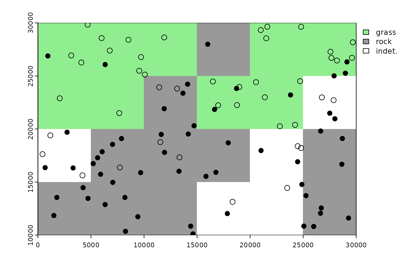
# plot environment classification vs. original points
plot(binRast, col = c('lightgreen', 'grey60', 'white'))
points(ptsDf[env=='rock', ], pch = 16, cex = 1.2) # occurrences of given habitat
points(ptsDf[env=='grass',], pch =  1, cex = 1.2)


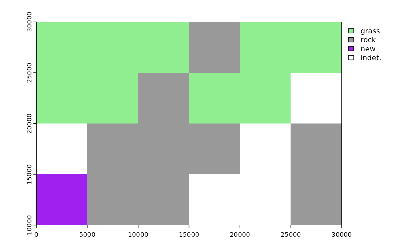
# classRast can also accept more than 2 environmental classes:

# add a 3rd environmental class with maximum occurrence in bottom-left grid cell
newEnv <- data.frame('x' = rep(0,       10),
                     'y' = rep(10000,   10),
                     'env' = rep('new', 10))
ptsDf <- rbind(ptsDf, newEnv)
binRast <- classRast(grid = r, dat = ptsDf, xy = c('x', 'y'),
                     env = 'env', cutoff = 0.6)
plot(binRast, col = c('lightgreen', 'grey60', 'purple', 'white'))